You are given an m x n integer matrix matrix with the following two properties:
Given an integer target, return true if target is in matrix or false otherwise.
You must write a solution in O(log(m * n)) time complexity.
Example 1:

Input: matrix = [[1,3,5,7],[10,11,16,20],[23,30,34,60]], target = 3
Output: true
Example 2:
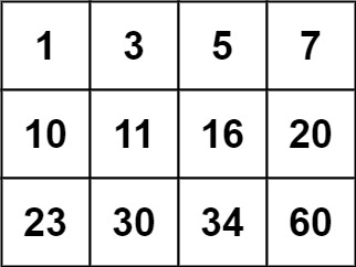
Input: matrix = [[1,3,5,7],[10,11,16,20],[23,30,34,60]], target = 13
Output: false
Constraints:
m == matrix.lengthn == matrix[i].length1 <= m, n <= 100-104 <= matrix[i][j], target <= 104Problem Overview: You are given an m x n matrix where each row is sorted in ascending order and the first element of each row is greater than the last element of the previous row. The task is to determine whether a given target value exists in the matrix.
Approach 1: Binary Search on Matrix as a 1D Array (O(log(m*n)) time, O(1) space)
The key insight is that the matrix behaves like a globally sorted array. Because every row starts with a value greater than the previous row’s last value, you can conceptually flatten the matrix into a single sorted list of size m * n. Run standard binary search on indices from 0 to m*n - 1. Convert a 1D index back to matrix coordinates using row = mid / n and col = mid % n. Each step compares matrix[row][col] with the target and halves the search space. This approach is optimal because it treats the structure as a single sorted dataset while keeping constant memory.
Approach 2: Two-step Binary Search (Row then Column) (O(log m + log n) time, O(1) space)
This method performs two separate binary searches. First, run binary search on the rows to locate the only row that could contain the target. Compare the target with the first and last element of each row to narrow down the candidate row. Once the correct row is identified, run a second binary search within that row to locate the target value. This approach explicitly uses the row ordering property of the matrix and the sorted order inside each row. It is easy to reason about during interviews because the two steps clearly mirror the structure of the data.
Both solutions rely on the same property: the matrix behaves like a sorted structure. The first approach compresses the entire matrix into a conceptual array, while the second approach searches rows and columns separately. Either way, the algorithm repeatedly halves the search space using array indexing and binary search comparisons.
Recommended for interviews: The 1D binary search approach is usually the expected optimal solution. It demonstrates that you recognize the matrix is globally sorted and can transform the problem into classic binary search. The two-step method is also accepted and often easier to derive during an interview because it directly uses the matrix layout.
The matrix can be viewed as a single sorted list. Hence, we can perform a binary search on the entire matrix by treating it as a 1D array. Suppose we have a matrix of size m x n, any element in the matrix can be accessed using a single index calculated as follows:
Element at index k can be accessed using matrix[k / n][k % n], where / and % represent integer division and modulus operations, respectively.
This approach ensures that the solution operates in O(log(m * n)) time complexity as required.
The function searchMatrix implements binary search on a conceptual 1D version of the matrix. The mid index is calculated using integer division and modulus to map it to the matrix cell. This mapping ensures that all matrix elements can be inspected via binary search.
Time complexity: O(log(m * n))
Space complexity: O(1)
The problem also allows for a two-step binary search owing to the special properties of the matrix. First, we identify the row which potentially contains the target by performing binary search on first elements of each row. Then, we conduct a binary search in that specific row.
Although not strictly O(log(m * n)), this approach exploits the matrix's properties in an efficient manner for similar effective results.
This C code expands the binary search to two distinct logical steps: first identifying the potential row and then binary searching within that row itself to find the target efficiently.
Time complexity: O(log(m) + log(n))
Space complexity: O(1)
We can logically unfold the two-dimensional matrix and then perform binary search.
The time complexity is O(log(m times n)), where m and n are the number of rows and columns of the matrix, respectively. The space complexity is O(1).
Python
Java
C++
Go
TypeScript
Rust
JavaScript
Here, we start searching from the bottom left corner and move towards the top right direction. We compare the current element matrix[i][j] with target:
matrix[i][j] = target, we have found the target value and return true.matrix[i][j] > target, all elements to the right of the current position in this row are greater than target, so we should move the pointer i upwards, i.e., i = i - 1.matrix[i][j] < target, all elements above the current position in this column are less than target, so we should move the pointer j to the right, i.e., j = j + 1.If we still can't find target after the search, return false.
The time complexity is O(m + n), where m and n are the number of rows and columns of the matrix, respectively. The space complexity is O(1).
| Approach | Complexity |
|---|---|
| Binary Search on Matrix as a 1D Array | Time complexity: |
| Two-step Binary Search (Row then Column) | Time complexity: |
| Binary Search | — |
| Search from the Bottom Left or Top Right | — |
| Approach | Time | Space | When to Use |
|---|---|---|---|
| Binary Search on Matrix as 1D Array | O(log(m*n)) | O(1) | Best general solution when the matrix behaves like a globally sorted array |
| Two-step Binary Search (Row then Column) | O(log m + log n) | O(1) | Useful when reasoning about row ranges first and then searching within a row |
Search a 2D Matrix - Leetcode 74 - Python • NeetCode • 261,802 views views
Watch 9 more video solutions →Practice Search a 2D Matrix with our built-in code editor and test cases.
Practice on FleetCodePractice this problem
Open in Editor