
Minimum Time to Visit Disappearing Nodes - Solution & Explanation
Problem Statement
There is an undirected graph of n nodes. You are given a 2D array edges, where edges[i] = [ui, vi, lengthi] describes an edge between node ui and node vi with a traversal time of lengthi units.
Additionally, you are given an array disappear, where disappear[i] denotes the time when the node i disappears from the graph and you won't be able to visit it.
Note that the graph might be disconnected and might contain multiple edges.
Return the array answer, with answer[i] denoting the minimum units of time required to reach node i from node 0. If node i is unreachable from node 0 then answer[i] is -1.
Example 1:
Input: n = 3, edges = [[0,1,2],[1,2,1],[0,2,4]], disappear = [1,1,5]
Output: [0,-1,4]
Explanation:
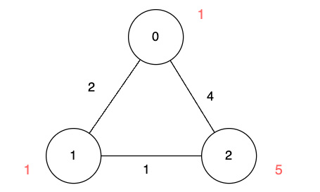
We are starting our journey from node 0, and our goal is to find the minimum time required to reach each node before it disappears.
- For node 0, we don't need any time as it is our starting point.
- For node 1, we need at least 2 units of time to traverse
edges[0]. Unfortunately, it disappears at that moment, so we won't be able to visit it. - For node 2, we need at least 4 units of time to traverse
edges[2].
Example 2:
Input: n = 3, edges = [[0,1,2],[1,2,1],[0,2,4]], disappear = [1,3,5]
Output: [0,2,3]
Explanation:
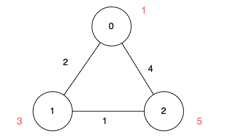
We are starting our journey from node 0, and our goal is to find the minimum time required to reach each node before it disappears.
- For node 0, we don't need any time as it is the starting point.
- For node 1, we need at least 2 units of time to traverse
edges[0]. - For node 2, we need at least 3 units of time to traverse
edges[0]andedges[1].
Example 3:
Input: n = 2, edges = [[0,1,1]], disappear = [1,1]
Output: [0,-1]
Explanation:
Exactly when we reach node 1, it disappears.
Constraints:
1 <= n <= 5 * 1040 <= edges.length <= 105edges[i] == [ui, vi, lengthi]0 <= ui, vi <= n - 11 <= lengthi <= 105disappear.length == n1 <= disappear[i] <= 105
Approach Overview
Problem Overview: You are given a weighted graph and an array disappear where each node becomes inaccessible after a specific time. Starting from node 0, compute the minimum time to reach every node before it disappears. If a node cannot be reached in time, its answer is -1.
Approach 1: Dijkstra's Algorithm with Disappearance Constraint (O((n+m) log n) time, O(n+m) space)
This problem behaves like a classic shortest path search with one extra rule: you cannot enter a node if the arrival time is greater than or equal to its disappearance time. Use Dijkstra’s algorithm with a heap (priority queue) to always process the node with the smallest current travel time. For each edge relaxation, compute next_time = current_time + weight and only push the neighbor if next_time < disappear[neighbor]. Maintain a distance array to avoid revisiting nodes with worse times. This approach works well because edge weights vary, and the priority queue guarantees the earliest feasible arrival is processed first.
Approach 2: Breadth-First Search with Edge Constraints (O(n+m) time, O(n+m) space)
If edge traversal behaves close to uniform or you structure the traversal level-by-level, a constrained BFS-style traversal can work. Store states in a queue and track the earliest time each node can be reached. When exploring neighbors, calculate the arrival time and skip the transition if the node would already have disappeared. This method still relies on pruning invalid states early and maintaining a visited or distance array to avoid redundant processing. Conceptually it treats the graph as layers of reachable states while enforcing the disappearance rule during expansion. It is useful for simpler implementations when edge weights or constraints allow near-linear traversal.
Recommended for interviews: Dijkstra’s algorithm is the expected solution. Interviewers want to see that you recognize the problem as a constrained graph shortest-path variant and modify the relaxation condition using the disappearance time. A brute traversal shows understanding of graph exploration, but the priority queue solution demonstrates mastery of shortest-path optimization.
Approach 1: Dijkstra's Algorithm with Constraints
Dijkstra's Algorithm with Constraints:
Use Dijkstra's algorithm to find the shortest paths from node 0 to all other nodes. However, during the traversal, consider the disappearance times of the nodes. If a node is reached after its disappearance time, consider it unreachable for that path.
This solution utilizes a modified version of Dijkstra's algorithm. The algorithm maintains a priority queue to ensure processing nodes with the least cumulative time first. Every time a node is dequeued, it checks if it was reached before its disappearance time. If not, it's effectively unreachable. This ensures all nodes that can be visited in time are correctly calculated.
Complexity
Time Complexity: O((n + e) log n), where n is the number of nodes and e is the number of edges.
Space Complexity: O(n + e), to store the graph and auxiliary data.
Approach 2: Breadth-First Search with Edge Constraints
Breadth-First Search with Edge Constraints:
Employ a breadth-first search (BFS) to explore the graph from the starting node. Use a queue to manage nodes to explore and ensure to update the shortest time to reach each node. Similar to Dijkstra, ensure that any node visited must be checked against its disappearance time to ensure the path is valid.
This C++ solution uses a BFS approach to explore the graph. A simple queue is used instead of a priority queue, but we must still ensure that paths followed are viable by checking the disappear quality of nodes. Similar to BFS, this approach traverses layer by layer in time when optimizing reachability.
Complexity
Time Complexity: O(n + e), because each node and edge is processed once.
Space Complexity: O(n + e), to store nodes and other state data.
Approach 3: Heap-Optimized Dijkstra
First, we create an adjacency list g to store the edges of the graph. Then, we create an array dist to store the shortest distances from node 0 to other nodes. Initialize dist[0] = 0, and the distances for the rest of the nodes are initialized to infinity.
Next, we use the Dijkstra algorithm to calculate the shortest distances from node 0 to other nodes. The specific steps are as follows:
- Create a priority queue
pqto store the distances and node numbers. Initially, add node0to the queue with a distance of0. - Remove a node
ufrom the queue. If the distanceduofuis greater thandist[u], it meansuhas already been updated, so we skip it directly. - Iterate through all neighbor nodes
vof nodeu. Ifdist[v] > dist[u] + wanddist[u] + w < disappear[v], then updatedist[v] = dist[u] + wand add nodevto the queue. - Repeat steps 2 and 3 until the queue is empty.
Finally, we iterate through the dist array. If dist[i] < disappear[i], then answer[i] = dist[i]; otherwise, answer[i] = -1.
The time complexity is O(m times log m), and the space complexity is O(m). Here, m is the number of edges.
Code
Python
Java
C++
Go
TypeScript
Complexity Comparison
| Approach | Complexity |
|---|---|
| Dijkstra's Algorithm with Constraints | Time Complexity: O((n + e) log n), where n is the number of nodes and e is the number of edges. |
| Breadth-First Search with Edge Constraints | Time Complexity: O(n + e), because each node and edge is processed once. |
| Heap-Optimized Dijkstra | — |
Detailed Complexity Analysis
| Approach | Time | Space | When to Use |
|---|---|---|---|
| Dijkstra's Algorithm with Disappearance Constraint | O((n+m) log n) | O(n+m) | General weighted graph case where edges have different travel times |
| Breadth-First Search with Edge Constraints | O(n+m) | O(n+m) | When traversal behaves close to uniform or constraints allow simple queue-based exploration |
Video Solution
3112. Minimum Time to Visit Disappearing Nodes | Dijkstras | Graph • Aryan Mittal • 2,775 views views
Watch 7 more video solutions →Frequently Asked Questions
Is Minimum Time to Visit Disappearing Nodes easy or hard?
Minimum Time to Visit Disappearing Nodes Python or Java solution
How to solve Minimum Time to Visit Disappearing Nodes in O(n log n)?
What is the best approach for Minimum Time to Visit Disappearing Nodes?
Is Minimum Time to Visit Disappearing Nodes asked at Google/Amazon/Meta?
What data structure is used in Minimum Time to Visit Disappearing Nodes?
What is the time complexity of Minimum Time to Visit Disappearing Nodes?
Ready to solve this problem?
Practice Minimum Time to Visit Disappearing Nodes with our built-in code editor and test cases.
Practice on FleetCodeProblem Info
Table of Contents
Practice this problem
Open in Editor