There is a country of n cities numbered from 0 to n - 1 where all the cities are connected by bi-directional roads. The roads are represented as a 2D integer array edges where edges[i] = [xi, yi, timei] denotes a road between cities xi and yi that takes timei minutes to travel. There may be multiple roads of differing travel times connecting the same two cities, but no road connects a city to itself.
Each time you pass through a city, you must pay a passing fee. This is represented as a 0-indexed integer array passingFees of length n where passingFees[j] is the amount of dollars you must pay when you pass through city j.
In the beginning, you are at city 0 and want to reach city n - 1 in maxTime minutes or less. The cost of your journey is the summation of passing fees for each city that you passed through at some moment of your journey (including the source and destination cities).
Given maxTime, edges, and passingFees, return the minimum cost to complete your journey, or -1 if you cannot complete it within maxTime minutes.
Example 1:
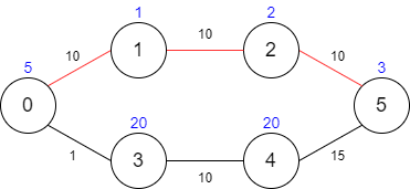
Input: maxTime = 30, edges = [[0,1,10],[1,2,10],[2,5,10],[0,3,1],[3,4,10],[4,5,15]], passingFees = [5,1,2,20,20,3]
Output: 11
Explanation: The path to take is 0 -> 1 -> 2 -> 5, which takes 30 minutes and has $11 worth of passing fees.
Example 2:
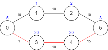
Input: maxTime = 29, edges = [[0,1,10],[1,2,10],[2,5,10],[0,3,1],[3,4,10],[4,5,15]], passingFees = [5,1,2,20,20,3]
Output: 48
Explanation: The path to take is 0 -> 3 -> 4 -> 5, which takes 26 minutes and has $48 worth of passing fees.
You cannot take path 0 -> 1 -> 2 -> 5 since it would take too long.
Example 3:
Input: maxTime = 25, edges = [[0,1,10],[1,2,10],[2,5,10],[0,3,1],[3,4,10],[4,5,15]], passingFees = [5,1,2,20,20,3]
Output: -1
Explanation: There is no way to reach city 5 from city 0 within 25 minutes.
Constraints:
1 <= maxTime <= 1000n == passingFees.length2 <= n <= 1000n - 1 <= edges.length <= 10000 <= xi, yi <= n - 11 <= timei <= 10001 <= passingFees[j] <= 1000 Problem Overview: You are given a graph where each city has a passing fee and each road has a travel time. Starting from city 0, reach city n-1 without exceeding maxTime. The goal is to minimize the total cost (sum of passing fees). If the destination cannot be reached within the allowed time, return -1.
This is a constrained shortest path problem. Traditional shortest path algorithms minimize either distance or cost, but here you must minimize cost while keeping total travel time ≤ maxTime. That constraint turns the problem into a hybrid of graph traversal and dynamic programming.
Approach 1: Dijkstra's Algorithm with Time Constraint (Time: O(E log V), Space: O(V * maxTime))
Treat each state as (city, timeSpent). Instead of tracking only the shortest distance, maintain the minimum cost required to reach a city at a specific time. Use a priority queue ordered by cost. From the current state, iterate over neighboring cities and push a new state if the updated time does not exceed maxTime. Maintain a DP table cost[city][time] to avoid revisiting worse states. This approach works because Dijkstra always expands the lowest-cost state first, ensuring that once the destination is reached within the allowed time, the cost is minimal. It performs well when the graph is sparse and is usually the fastest solution in practice.
Approach 2: Bellman-Ford Style Dynamic Programming (Time: O(maxTime * E), Space: O(V))
Another way is to iterate over time like a dynamic programming dimension. Maintain an array where dp[i] stores the minimum cost to reach city i. For each time unit up to maxTime, relax all edges. When relaxing an edge (u → v) with travel time t, update the cost for reaching v if the total time stays within the limit. To avoid overwriting values in the same iteration, copy the previous DP state before relaxing edges. This approach resembles the Bellman-Ford algorithm applied across time layers and works well for dense graphs. It explicitly explores all feasible transitions without using a priority queue.
Both solutions rely on modeling the graph using adjacency lists built from the input arrays. The key insight is that the same city can be visited multiple times if the arrival time differs, because a later arrival might still produce a cheaper total cost.
Recommended for interviews: Dijkstra with a time constraint is the preferred solution. Interviewers expect you to recognize this as a shortest-path problem with an additional state dimension. The Bellman-Ford style DP demonstrates strong understanding of relaxation techniques and constrained path problems, but the priority-queue solution is usually considered the optimal and most scalable approach.
This approach uses a variation of Dijkstra's algorithm to find the path with the minimum cost. While standard Dijkstra's algorithm optimizes for the shortest path, here, we will need to consider both the cost and the time constraints.
We will use a priority queue to focus on minimizing cost, and keep an array to track the minimum time to reach each city. If a city can be reached with a lesser cost within the allowed time, we choose that path. This approach involves maintaining additional state for the journey's time and cost.
This implementation uses an array as a priority queue to maintain the state of each city visit with cost and time. When a new city visit results in a lower cost within the allowed time, it adds that state to the queue. The priority queue is implemented as a simple array sorted for minimal cost retrieval.
Time Complexity: O(E log V), where E is the number of edges and V is the number of vertices. Sorting the array incurs additional complexity, but the algorithm prioritizes cost over time.
Space Complexity: O(V + E), storing the state for each vertex in the graph and the priority queue.
The Bellman-Ford algorithm is apt for graphs with cycles and works generally well especially when negative weights might be a consideration (not in this problem though). It checks all edges repeatedly to relax them and can accommodate additional constraints by modifying its relaxations - here, including time tracking for paths.
This implementation facilitates edge relaxation through maximum iterations to ensure paths of lesser costs are rendered consistently. The solution extends Bellman-Ford provisions to preclude infeasible paths by scrutinizing time consumption contradicting allowed limits.
Time Complexity: O(V * E), where V is the number of vertices and E is the number of edges.
Space Complexity: O(V), with storage necessary for resultant paths and critical costs.
We define f[i][j] to represent the minimum cost to reach city j from city 0 after i minutes. Initially, f[0][0] = passingFees[0], and the rest f[0][j] = +infty.
Next, within the time range [1, maxTime], we traverse all edges. For each edge (x, y, t), if t leq i, then we:
i - t minutes to reach city y from city 0, then spend t minutes to reach city x from city y, and add the passing fee to reach city x, i.e., f[i][x] = min(f[i][x], f[i - t][y] + passingFees[x]);i - t minutes to reach city x from city 0, then spend t minutes to reach city y from city x, and add the passing fee to reach city y, i.e., f[i][y] = min(f[i][y], f[i - t][x] + passingFees[y]).The final answer is min{f[i][n - 1]}, where i \in [0, maxTime]. If the answer is +infty, return -1.
The time complexity is O(maxTime times (m + n)), where m and n are the number of edges and cities, respectively. The space complexity is O(maxTime times n).
Python
Java
C++
Go
TypeScript
| Approach | Complexity |
|---|---|
| Dijkstra's Algorithm with Time Constraint | Time Complexity: O(E log V), where E is the number of edges and V is the number of vertices. Sorting the array incurs additional complexity, but the algorithm prioritizes cost over time. Space Complexity: O(V + E), storing the state for each vertex in the graph and the priority queue. |
| Bellman-Ford Algorithm with Time Cost | Time Complexity: O(V * E), where V is the number of vertices and E is the number of edges. Space Complexity: O(V), with storage necessary for resultant paths and critical costs. |
| Dynamic Programming | — |
| Approach | Time | Space | When to Use |
|---|---|---|---|
| Dijkstra's Algorithm with Time Constraint | O(E log V) | O(V * maxTime) | Best general solution for sparse graphs and interview settings. Efficient with priority queue pruning. |
| Bellman-Ford Dynamic Programming | O(maxTime * E) | O(V) | Useful when modeling time as a DP dimension or when avoiding priority queues. |
LeetCode 1928. Minimum Cost to Reach Destination in Time • Happy Coding • 4,960 views views
Watch 9 more video solutions →Practice Minimum Cost to Reach Destination in Time with our built-in code editor and test cases.
Practice on FleetCode