
Maximum Number of Moves in a Grid - Solution & Explanation
Problem Statement
You are given a 0-indexed m x n matrix grid consisting of positive integers.
You can start at any cell in the first column of the matrix, and traverse the grid in the following way:
- From a cell
(row, col), you can move to any of the cells:(row - 1, col + 1),(row, col + 1)and(row + 1, col + 1)such that the value of the cell you move to, should be strictly bigger than the value of the current cell.
Return the maximum number of moves that you can perform.
Example 1:
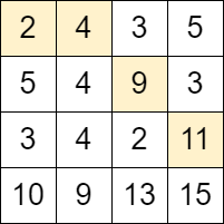
Input: grid = [[2,4,3,5],[5,4,9,3],[3,4,2,11],[10,9,13,15]]
Output: 3
Explanation: We can start at the cell (0, 0) and make the following moves:
- (0, 0) -> (0, 1).
- (0, 1) -> (1, 2).
- (1, 2) -> (2, 3).
It can be shown that it is the maximum number of moves that can be made.
Example 2:
Input: grid = [[3,2,4],[2,1,9],[1,1,7]]
Output: 0
Explanation: Starting from any cell in the first column we cannot perform any moves.
Constraints:
m == grid.lengthn == grid[i].length2 <= m, n <= 10004 <= m * n <= 1051 <= grid[i][j] <= 106
Approach Overview
Problem Overview: You are given an m x n grid of integers. Starting from any cell in the first column, you can move to (row-1, col+1), (row, col+1), or (row+1, col+1) if the destination value is strictly greater than the current cell. The task is to compute the maximum number of moves possible following these rules.
Approach 1: Divide and Conquer with DFS + Memoization (O(m * n) time, O(m * n) space)
Treat each cell as the start of a subproblem: the maximum moves you can make beginning from that position. From cell (r, c), recursively explore the three valid next positions in column c + 1 that contain larger values. Without caching, this would recompute the same paths many times. Memoization stores the result for each cell so every state is solved once. The recursion effectively performs a depth‑first search across the grid while caching results in a DP table. This approach maps naturally to dynamic programming over a matrix, and the state transition simply picks the best of the three possible moves.
Approach 2: Iterative Subproblem Solving (Bottom‑Up DP) (O(m * n) time, O(m * n) space)
The recursive solution can be converted into a bottom‑up DP. Process columns from right to left since moves always go to col + 1. Maintain a DP table where dp[r][c] represents the maximum moves starting from cell (r, c). For each cell, check the three possible neighbors in the next column. If the neighbor’s value is larger, update dp[r][c] = 1 + dp[next]. The answer is the maximum value among all cells in the first column. This avoids recursion overhead and keeps the transition logic explicit. Iterating column by column also makes boundary handling easier when working with arrays and grids.
Recommended for interviews: The DFS + memoization approach clearly shows the state transition and demonstrates strong understanding of dynamic programming on grids. Interviewers often expect you to first describe the recursive exploration and then optimize it with memoization. The bottom‑up DP version shows additional maturity by eliminating recursion and computing the same states iteratively.
Approach 1: Divide and Conquer
This approach involves breaking down the problem into smaller subproblems. Each subproblem is solved independently, and the solutions to these subproblems are combined to solve the original problem. This is typically implemented through recursive functions.
This C program uses a divide and conquer strategy to solve the problem. The solveSubProblem function is called recursively to divide the data array until each subproblem reaches a base case (when start is greater than or equal to end). After each recursion, it combines results of the subproblems to form a contiguous solution. You will need to fill in the logic to solve your specific problem within the 'Combine results' section.
Complexity
Time Complexity: O(n log n) due to the divide and conquer methodology where the problem is divided into two halves.
Space Complexity: O(log n) due to the recursive stack depth.
Approach 2: Iterative Subproblem Solving
This approach avoids recursion by iteratively solving subproblems. It may use data structures as stacks or queues to keep track of subproblems, or directly manipulate indices to iterate over sections of the data.
This C implementation replaces recursion with iteration, analyzing subproblems iteratively and solving them in sequence. There will need to be a clear method for handling and processing each segment of the data.
Complexity
Time Complexity: O(n), if the problem can be iteratively solved in linear time.
Space Complexity: O(1), if no extra storage apart from input data is used.
Approach 3: BFS
We define a queue q, and initially add all the row coordinates of the first column to the queue.
Next, we start from the first column and traverse column by column. For each column, we take out all the row coordinates in the queue one by one. For each row coordinate i, we get all possible row coordinates k of the next column, and satisfy grid[i][j] < grid[k][j + 1], and add these row coordinates to a new set t. If t is empty, it means that we cannot continue to move, so we return the current column number. Otherwise, we assign t to q and continue to traverse the next column.
Finally, if we have traversed all the columns, it means that we can move to the last column, so we return n - 1.
The time complexity is O(m times n), and the space complexity is O(m). Where m and n are the number of rows and columns in the matrix, respectively.
Code
Python
Java
C++
Go
TypeScript
Complexity Comparison
| Approach | Complexity |
|---|---|
| Divide and Conquer | Time Complexity: O(n log n) due to the divide and conquer methodology where the problem is divided into two halves. |
| Iterative Subproblem Solving | Time Complexity: O(n), if the problem can be iteratively solved in linear time. |
| BFS | — |
Detailed Complexity Analysis
| Approach | Time | Space | When to Use |
|---|---|---|---|
| Divide and Conquer (DFS + Memoization) | O(m * n) | O(m * n) | When modeling the problem recursively or explaining the DP state transition during interviews |
| Iterative Subproblem Solving (Bottom-Up DP) | O(m * n) | O(m * n) | When you want an iterative solution without recursion overhead and clearer DP table updates |
Video Solution
Maximum Number of Moves in a Grid | Simplest Approach | Leetcode 2684 | codestorywithMIK • codestorywithMIK • 6,425 views views
Watch 9 more video solutions →Frequently Asked Questions
Is Maximum Number of Moves in a Grid easy or hard?
How to solve Maximum Number of Moves in a Grid in O(m * n)?
What is the best approach for Maximum Number of Moves in a Grid?
Is Maximum Number of Moves in a Grid asked at Google/Amazon/Meta?
What data structure is used in Maximum Number of Moves in a Grid?
What is the time complexity of Maximum Number of Moves in a Grid?
Maximum Number of Moves in a Grid Python or Java solution approach?
Ready to solve this problem?
Practice Maximum Number of Moves in a Grid with our built-in code editor and test cases.
Practice on FleetCodeTable of Contents
Practice this problem
Open in Editor