Given an m x n binary matrix filled with 0's and 1's, find the largest square containing only 1's and return its area.
Example 1:
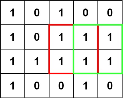
Input: matrix = [["1","0","1","0","0"],["1","0","1","1","1"],["1","1","1","1","1"],["1","0","0","1","0"]]
Output: 4
Example 2:

Input: matrix = [["0","1"],["1","0"]]
Output: 1
Example 3:
Input: matrix = [["0"]]
Output: 0
Constraints:
m == matrix.lengthn == matrix[i].length1 <= m, n <= 300matrix[i][j] is '0' or '1'.Problem Overview: You receive a binary matrix of '0' and '1'. The goal is to find the largest square containing only 1s and return its area. The challenge is detecting square expansion efficiently instead of checking every possible submatrix.
Approach 1: Dynamic Programming (O(m*n) time, O(m*n) space)
The key observation: a square ending at cell (i, j) can only grow if the three neighboring squares (i-1, j), (i, j-1), and (i-1, j-1) also support that expansion. Define dp[i][j] as the side length of the largest square whose bottom-right corner is at (i, j). If the matrix value is '1', compute dp[i][j] = 1 + min(top, left, diagonal). If it is '0', the value stays 0. While iterating through the matrix row by row, track the maximum side length seen so far and square it at the end to get the area. This approach transforms a brute-force square validation problem into a local recurrence using dynamic programming. Time complexity is O(m*n) because every cell is processed once. Space complexity is O(m*n) for the DP table.
Approach 2: Space Optimized DP (O(m*n) time, O(n) space)
The full DP table is not strictly required because each state depends only on the previous row and the current row. Instead of storing the entire matrix of DP states, maintain a single array representing the previous row plus a variable for the diagonal value. While iterating through columns, update the current cell using the same recurrence: 1 + min(top, left, diagonal). The trick is preserving the old value of dp[j] before overwriting it so it can act as the diagonal for the next computation. This reduces memory usage significantly while preserving the same logic. Time complexity remains O(m*n), but space drops to O(n), where n is the number of columns.
Both approaches rely on scanning the grid and updating state based on neighboring cells, a common pattern in matrix and array DP problems. The recurrence works because a larger square can only exist if all three adjacent smaller squares already exist.
Recommended for interviews: The standard dynamic programming approach is what interviewers typically expect. Explaining the recurrence dp[i][j] = 1 + min(top, left, diagonal) demonstrates understanding of 2D DP state transitions. After presenting that solution, mentioning the space optimization to O(n) shows deeper mastery and awareness of practical constraints.
In this approach, a dynamic programming (DP) table is used to store the size of the largest square whose bottom-right corner is at each cell. For each cell (i, j) with a value of '1', we check its top (i-1, j), left (i, j-1), and top-left (i-1, j-1) neighbors to determine the size of the largest square ending at (i, j). If any of these neighbors are '0', the square cannot extend to include (i, j). The formula is: dp[i][j] = min(dp[i-1][j], dp[i][j-1], dp[i-1][j-1]) + 1. The maximum value in the DP table will be the side length of the largest square, and the area is its square.
The Python solution initializes a DP table with one extra row and column filled with zeros, to handle boundary conditions without additional checks. It iterates through the matrix, updating the DP table using the given formula and tracking the maximum square side found.
Time Complexity: O(m * n), where m is the number of rows and n is the number of columns.
Space Complexity: O(m * n), due to the DP table.
This approach uses a similar DP strategy but optimizes space by utilizing a one-dimensional array instead of a full 2D DP table. The key idea is that while processing the matrix row by row, previous rows' information will be partially redundant. Hence, we can maintain only the current and previous row data in separate arrays or even use a single array with swap states.
The space-optimized Python solution uses two arrays; one for the current row calculations and one for the previous row's data. After finishing each row, it swaps the references, reassigning the current as 'previous'. This approach reduces space use to O(n).
Time Complexity: O(m * n)
Space Complexity: O(n)
| Approach | Complexity |
|---|---|
| Dynamic Programming Approach | Time Complexity: O(m * n), where m is the number of rows and n is the number of columns. |
| Space Optimized DP Approach | Time Complexity: O(m * n) |
| Approach | Time | Space | When to Use |
|---|---|---|---|
| Dynamic Programming (2D DP Table) | O(m*n) | O(m*n) | Best for clarity during interviews and when memory usage is not a concern |
| Space Optimized DP | O(m*n) | O(n) | Preferred when matrix is large and memory optimization matters |
Maximal Square - Top Down Memoization - Leetcode 221 • NeetCode • 104,006 views views
Watch 9 more video solutions →Practice Maximal Square with our built-in code editor and test cases.
Practice on FleetCodePractice this problem
Open in Editor