You are given a positive integer n, indicating that we initially have an n x n 0-indexed integer matrix mat filled with zeroes.
You are also given a 2D integer array query. For each query[i] = [row1i, col1i, row2i, col2i], you should do the following operation:
1 to every element in the submatrix with the top left corner (row1i, col1i) and the bottom right corner (row2i, col2i). That is, add 1 to mat[x][y] for all row1i <= x <= row2i and col1i <= y <= col2i.Return the matrix mat after performing every query.
Example 1:
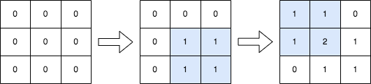
Input: n = 3, queries = [[1,1,2,2],[0,0,1,1]]
Output: [[1,1,0],[1,2,1],[0,1,1]]
Explanation: The diagram above shows the initial matrix, the matrix after the first query, and the matrix after the second query.
- In the first query, we add 1 to every element in the submatrix with the top left corner (1, 1) and bottom right corner (2, 2).
- In the second query, we add 1 to every element in the submatrix with the top left corner (0, 0) and bottom right corner (1, 1).
Example 2:
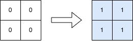
Input: n = 2, queries = [[0,0,1,1]]
Output: [[1,1],[1,1]]
Explanation: The diagram above shows the initial matrix and the matrix after the first query.
- In the first query we add 1 to every element in the matrix.
Constraints:
1 <= n <= 5001 <= queries.length <= 1040 <= row1i <= row2i < n0 <= col1i <= col2i < nProblem Overview: You are given an n x n matrix initially filled with zeros and a list of queries. Each query defines a submatrix using coordinates [r1, c1, r2, c2]. Every cell inside that rectangle must be incremented by one. After processing all queries, return the final matrix.
Approach 1: Naive Simulation (Time: O(q * n^2), Space: O(1) extra)
The most direct solution simulates each query exactly as described. For every query, iterate through rows from r1 to r2 and columns from c1 to c2, incrementing each cell by one. The implementation is straightforward and useful when constraints are small. However, if the matrix is large or the number of queries grows, this becomes expensive because each query may touch up to n^2 cells.
This approach works as a baseline to confirm correctness but does not scale well. In worst cases with thousands of queries and large matrices, repeated updates dominate runtime.
Approach 2: 2D Difference Array + Prefix Sum (Time: O(n^2 + q), Space: O(n^2))
The optimal approach avoids updating every cell of a submatrix individually. Instead, treat each update as a boundary operation using a 2D difference array. For a query [r1, c1, r2, c2], apply four corner updates:
diff[r1][c1] += 1diff[r1][c2 + 1] -= 1diff[r2 + 1][c1] -= 1diff[r2 + 1][c2 + 1] += 1
These operations mark where increments start and stop. After processing all queries, compute a 2D prefix sum over the matrix to propagate the increments to every affected cell. Each cell accumulates contributions from previous rows and columns, producing the final grid.
This technique is a classic extension of the difference-array idea commonly used in array problems. The prefix propagation step relies on concepts from prefix sum computation applied over a matrix. Instead of repeatedly modifying large regions, you convert each query into constant-time boundary updates.
The result is a major improvement: queries cost O(1) each, and the final reconstruction costs O(n^2). This makes the approach efficient even when the query list is large.
Recommended for interviews: Interviewers expect the prefix sum optimization. Implementing the naive simulation first shows you understand the problem mechanics. Recognizing that repeated region updates can be replaced with a difference array demonstrates deeper algorithmic thinking and familiarity with range-update techniques.
This approach involves directly iterating over each query and incrementing the submatrices defined by each query one element at a time. The advantage is simplicity, though it may not be optimal for larger matrices.
This code iterates through each provided query, applying a straightforward nested loop over the submatrix defined by each query, incrementing each element directly. This is simple but can be slow for large matrices due to the repeated traversal.
Time Complexity: O(n * queries.length * n) since for each query we potentially look at n^2 elements.
Space Complexity: O(n^2) for the matrix itself.
This optimized approach involves utilizing a technique akin to prefix sums. By marking only changes at the boundaries of the submatrix, we can later apply a prefix sum over the matrix to effectively accumulate the desired increments.
The optimized C solution uses auxiliary plus signs for boundaries to demarcate increments, followed by a prefix sum application on mat, building the desired output efficiently.
Time Complexity: O(n^2) due to prefix sum computations.
Space Complexity: O(n^2) for the augmented storage of the matrix.
A 2D difference array is a technique used to efficiently handle range updates on 2D arrays. We can implement fast updates on submatrices by maintaining a difference matrix of the same size as the original matrix.
Suppose we have a 2D difference matrix diff, initially with all elements set to 0. For each query [row1, col1, row2, col2], we can update the difference matrix through the following steps:
(row1, col1) by 1.(row2 + 1, col1) by 1, provided that row2 + 1 < n.(row1, col2 + 1) by 1, provided that col2 + 1 < n.(row2 + 1, col2 + 1) by 1, provided that row2 + 1 < n and col2 + 1 < n.After completing all queries, we need to convert the difference matrix back to the original matrix using prefix sums. That is, for each position (i, j), we calculate:
$
mat[i][j] = diff[i][j] + (mat[i-1][j] if i > 0 else 0) + (mat[i][j-1] if j > 0 else 0) - (mat[i-1][j-1] if i > 0 and j > 0 else 0)
The time complexity is O(m + n^2), where m and n are the length of queries and the given n, respectively. Ignoring the space consumed by the answer, the space complexity is O(1)$.
| Approach | Complexity |
|---|---|
| Naive Approach | Time Complexity: O(n * queries.length * n) since for each query we potentially look at n^2 elements. |
| Prefix Sum Approach (Optimization) | Time Complexity: O(n^2) due to prefix sum computations. |
| 2D Difference Array | — |
| Approach | Time | Space | When to Use |
|---|---|---|---|
| Naive Simulation | O(q * n^2) | O(1) | Small matrices or when demonstrating the straightforward logic first |
| 2D Difference Array + Prefix Sum | O(n^2 + q) | O(n^2) | Large number of queries or interview settings requiring optimized range updates |
Increment Submatrices by One | Difference Array Technique in 2-D Array | Leetcode 2536 | MIK • codestorywithMIK • 7,186 views views
Watch 9 more video solutions →Practice Increment Submatrices by One with our built-in code editor and test cases.
Practice on FleetCodePractice this problem
Open in Editor