You are given a rows x cols matrix grid representing a field of cherries where grid[i][j] represents the number of cherries that you can collect from the (i, j) cell.
You have two robots that can collect cherries for you:
(0, 0), and(0, cols - 1).Return the maximum number of cherries collection using both robots by following the rules below:
(i, j), robots can move to cell (i + 1, j - 1), (i + 1, j), or (i + 1, j + 1).grid.
Example 1:
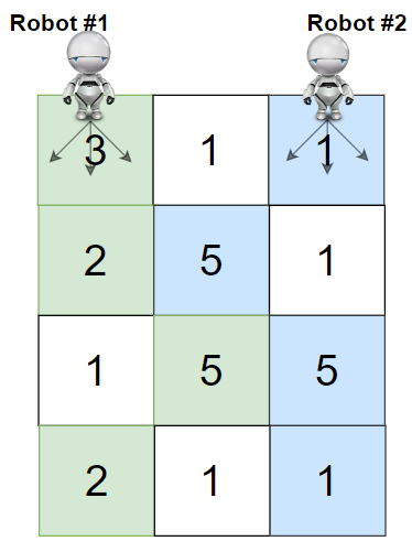
Input: grid = [[3,1,1],[2,5,1],[1,5,5],[2,1,1]]
Output: 24
Explanation: Path of robot #1 and #2 are described in color green and blue respectively.
Cherries taken by Robot #1, (3 + 2 + 5 + 2) = 12.
Cherries taken by Robot #2, (1 + 5 + 5 + 1) = 12.
Total of cherries: 12 + 12 = 24.
Example 2:
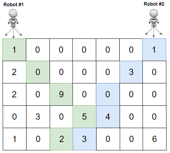
Input: grid = [[1,0,0,0,0,0,1],[2,0,0,0,0,3,0],[2,0,9,0,0,0,0],[0,3,0,5,4,0,0],[1,0,2,3,0,0,6]]
Output: 28
Explanation: Path of robot #1 and #2 are described in color green and blue respectively.
Cherries taken by Robot #1, (1 + 9 + 5 + 2) = 17.
Cherries taken by Robot #2, (1 + 3 + 4 + 3) = 11.
Total of cherries: 17 + 11 = 28.
Constraints:
rows == grid.lengthcols == grid[i].length2 <= rows, cols <= 700 <= grid[i][j] <= 100Problem Overview: You control two robots starting at the top row of a grid. One begins at the leftmost column and the other at the rightmost column. Each step both robots move to the next row and can shift left, stay, or shift right. The goal is to collect the maximum number of cherries while ensuring a cell's cherries are counted once if both robots land on it.
Approach 1: Recursive Approach with Memoization (Time: O(rows * cols²), Space: O(rows * cols²))
Model the problem using a recursive state (row, col1, col2) representing the current row and the column positions of both robots. From this state, explore all 9 possible next moves because each robot can move to col-1, col, or col+1. Add cherries from the current cells and recursively compute the best outcome for the next row. Without caching, the search explodes exponentially. Memoization stores results for each state so repeated subproblems are reused. A 3D memo table or hash map avoids recomputation and keeps the complexity bounded. This approach maps naturally to the problem definition and is often the easiest way to derive the correct transition logic.
Approach 2: Dynamic Programming (Bottom-Up) (Time: O(rows * cols²), Space: O(rows * cols²))
The optimized solution converts the recursive idea into bottom-up dynamic programming. Define dp[row][c1][c2] as the maximum cherries collected when robot1 is at column c1 and robot2 is at column c2 on a given row. Iterate row by row through the matrix. For each pair of columns, compute the best value from the 9 previous column combinations. Add cherries from grid[row][c1] and grid[row][c2], making sure to count only once if c1 == c2. This DP effectively tracks both robots simultaneously while exploring all movement combinations. Since there are rows levels and roughly cols² column pairs per level, the total work stays manageable.
The key insight is that both robots always move downward together. That means the row index is shared, reducing the state to three variables instead of tracking full paths. Treating the robots' positions as a pair avoids double counting and keeps transitions local to the previous row.
Recommended for interviews: The bottom-up dynamic programming approach is what most interviewers expect. It demonstrates that you can convert a recursive state definition into an efficient tabulation strategy. Starting with the memoized recursion shows understanding of the state transition, while implementing the DP version proves you can optimize overlapping subproblems. Problems involving two agents moving through a grid commonly appear in array and DP interview rounds, especially when the solution requires multi-dimensional state design.
This approach involves using a dynamic programming table to store intermediate results. The state dp[r][c1][c2] represents the maximum cherries we can collect when robot 1 is at position (r, c1) and robot 2 is at (r, c2). The transition involves moving both robots to the next row and trying all possible column moves for each robot.
This function implements a dynamic programming solution. We use a 3D table dp where dp[r][c1][c2] represents the maximum cherries obtainable starting from row r with robot 1 at column c1 and robot 2 at column c2. We transition backwards from the last row to the first row, checking all possible moves for the robots.
Time Complexity: O(rows * cols^2)
Space Complexity: O(rows * cols^2)
This approach uses a recursive function with memoization to calculate the maximum cherries possible. The function recursively tries all valid ways the robots can move to the next row from their current columns, caching results to prevent redundant calculations.
The Java solution uses recursion with memoization, where dfs is the recursive function that calculates the maximum cherries possible from any given position, storing results in memo to optimize repeat calculations. Each call considers new positions for the robots in the next row.
Java
JavaScript
Time Complexity: O(rows * cols^2)
Space Complexity: O(rows * cols^2) for memoization
We define f[i][j_1][j_2] as the maximum number of cherries that can be picked when the two robots are at positions j_1 and j_2 in the i-th row. Initially, f[0][0][n-1] = grid[0][0] + grid[0][n-1], and the other values are -1. The answer is max_{0 leq j_1, j_2 < n} f[m-1][j_1][j_2].
Consider f[i][j_1][j_2]. If j_1 neq j_2, then the number of cherries that the robots can pick in the i-th row is grid[i][j_1] + grid[i][j_2]. If j_1 = j_2, then the number of cherries that the robots can pick in the i-th row is grid[i][j_1]. We can enumerate the previous state of the two robots f[i-1][y1][y2], where y_1, y_2 are the positions of the two robots in the (i-1)-th row, then y_1 \in {j_1-1, j_1, j_1+1} and y_2 \in {j_2-1, j_2, j_2+1}. The state transition equation is as follows:
$
f[i][j_1][j_2] = max_{y_1 \in {j_1-1, j_1, j_1+1}, y_2 \in {j_2-1, j_2, j_2+1}} f[i-1][y_1][y_2] + \begin{cases} grid[i][j_1] + grid[i][j_2], & j_1 neq j_2 \ grid[i][j_1], & j_1 = j_2 \end{cases}
Where f[i-1][y_1][y_2] is ignored when it is -1.
The final answer is max_{0 leq j_1, j_2 < n} f[m-1][j_1][j_2].
The time complexity is O(m times n^2), and the space complexity is O(m times n^2). Where m and n$ are the number of rows and columns of the grid, respectively.
Python
Java
C++
Go
TypeScript
Notice that the calculation of f[i][j_1][j_2] is only related to f[i-1][y_1][y_2]. Therefore, we can use a rolling array to optimize the space complexity. After optimizing the space complexity, the time complexity is O(n^2).
Python
Java
C++
Go
TypeScript
| Approach | Complexity |
|---|---|
| Dynamic Programming Approach | Time Complexity: O(rows * cols^2) |
| Recursive Approach with Memoization | Time Complexity: O(rows * cols^2) |
| Dynamic Programming | — |
| Dynamic Programming (Space Optimization) | — |
| Approach | Time | Space | When to Use |
|---|---|---|---|
| Recursive with Memoization | O(rows * cols²) | O(rows * cols²) | Best for understanding the state transition and deriving the recurrence relation |
| Bottom-Up Dynamic Programming | O(rows * cols²) | O(rows * cols²) | Preferred production and interview solution with predictable iteration and no recursion overhead |
DP 13. Cherry Pickup II | 3D DP Made Easy | DP On Grids • take U forward • 377,912 views views
Watch 9 more video solutions →Practice Cherry Pickup II with our built-in code editor and test cases.
Practice on FleetCode