There exists an undirected and initially unrooted tree with n nodes indexed from 0 to n - 1. You are given the integer n and a 2D integer array edges of length n - 1, where edges[i] = [ai, bi] indicates that there is an edge between nodes ai and bi in the tree.
Each node has an associated price. You are given an integer array price, where price[i] is the price of the ith node.
The price sum of a given path is the sum of the prices of all nodes lying on that path.
The tree can be rooted at any node root of your choice. The incurred cost after choosing root is the difference between the maximum and minimum price sum amongst all paths starting at root.
Return the maximum possible cost amongst all possible root choices.
Example 1:
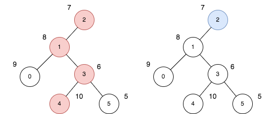
Input: n = 6, edges = [[0,1],[1,2],[1,3],[3,4],[3,5]], price = [9,8,7,6,10,5]
Output: 24
Explanation: The diagram above denotes the tree after rooting it at node 2. The first part (colored in red) shows the path with the maximum price sum. The second part (colored in blue) shows the path with the minimum price sum.
- The first path contains nodes [2,1,3,4]: the prices are [7,8,6,10], and the sum of the prices is 31.
- The second path contains the node [2] with the price [7].
The difference between the maximum and minimum price sum is 24. It can be proved that 24 is the maximum cost.
Example 2:
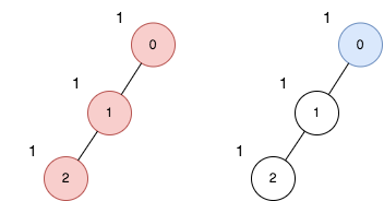
Input: n = 3, edges = [[0,1],[1,2]], price = [1,1,1]
Output: 2
Explanation: The diagram above denotes the tree after rooting it at node 0. The first part (colored in red) shows the path with the maximum price sum. The second part (colored in blue) shows the path with the minimum price sum.
- The first path contains nodes [0,1,2]: the prices are [1,1,1], and the sum of the prices is 3.
- The second path contains node [0] with a price [1].
The difference between the maximum and minimum price sum is 2. It can be proved that 2 is the maximum cost.
Constraints:
1 <= n <= 105edges.length == n - 10 <= ai, bi <= n - 1edges represents a valid tree.price.length == n1 <= price[i] <= 105The key observation for #2538 Difference Between Maximum and Minimum Price Sum is that the input forms a tree, so every pair of nodes has a unique path. The goal is to maximize the difference between two valid price sums that originate from the same chosen root.
A common strategy is to use Depth-First Search (DFS) combined with tree dynamic programming. For each node, compute two states: the best downward path sum that must end at a leaf and another that represents the best path that can stop at any node. While traversing children, we combine these values to update the global maximum difference.
This approach efficiently propagates optimal partial results up the tree. Since each edge and node is processed a constant number of times during DFS, the algorithm runs in O(n) time with O(n) space for recursion and adjacency structures.
| Approach | Time Complexity | Space Complexity |
|---|---|---|
| DFS with Tree Dynamic Programming | O(n) | O(n) |
Sahil & Sarra
Use these hints if you're stuck. Try solving on your own first.
The minimum price sum is always the price of a rooted node.
Let’s root the tree at vertex 0 and find the answer from this perspective.
In the optimal answer maximum price is the sum of the prices of nodes on the path from “u” to “v” where either “u” or “v” is the parent of the second one or neither is a parent of the second one.
The first case is easy to find. For the second case, notice that in the optimal path, “u” and “v” are both leaves. Then we can use dynamic programming to find such a path.
Let DP(v,1) denote “the maximum price sum from node v to leaf, where v is a parent of that leaf” and let DP(v,0) denote “the maximum price sum from node v to leaf, where v is a parent of that leaf - price[leaf]”. Then the answer is maximum of DP(u,0) + DP(v,1) + price[parent] where u, v are directly connected to vertex “parent”.
Watch expert explanations and walkthroughs
Practice problems asked by these companies to ace your technical interviews.
Explore More ProblemsJot down your thoughts, approach, and key learnings
DFS naturally explores hierarchical structures like trees and allows results from child nodes to be propagated back to the parent. This makes it ideal for computing downward path sums and combining subtree information during dynamic programming.
Problems involving tree DP and path optimization are common in FAANG-style interviews. While this exact question may not always appear, similar concepts such as DFS on trees, rerooting techniques, and path sum optimization are frequently tested.
An adjacency list is the best structure to represent the tree because it allows efficient traversal of neighbors. It works well with DFS-based dynamic programming and keeps the overall complexity linear in the number of nodes.
The optimal approach uses Depth-First Search with tree dynamic programming. For each node, you track the best path that must end at a leaf and another that can stop anywhere. Combining these values while traversing the tree helps compute the maximum possible difference efficiently.