
Minimum Time to Reach Target With Limited Power - Video Solutions
Leetcode 3977 | Minimum Time to Reach Target With Limited Power | Dijkstra | Weekly contest 508
Minimum Time to Reach Target With Limited Power - Video Solution
Watch 2 video solutions for Minimum Time to Reach Target With Limited Power, a hard level problem involving Array, Dynamic Programming, Graph. This walkthrough by CodeWithMeGuys has 215 views views. Want to try solving it yourself? Practice on FleetCode or read the detailed text solution.
Problem Statement
You are given a directed weighted graph with n nodes labeled from 0 to n - 1.
The graph is represented by a 2D integer array edges, where edges[i] = [ui, vi, ti] indicates a directed edge from node ui to node vi that takes ti seconds to traverse.
You are also given an integer power representing the initial available power, and an integer array cost of length n, where cost[u] represents the power required to forward the signal from node u through any one of its outgoing edges.
You are given two integers source and target.
The signal starts at source at time 0 with power units of power and follows these rules:
- The signal may traverse a directed edge from node
uonly if the remaining power is at leastcost[u]. - No power is consumed when the signal arrives at a node, unless it later leaves that node by traversing another edge.
- When the signal is forwarded from node
u, the remaining power is decreased bycost[u]units. - Traversing an edge
edges[i] = [ui, vi, ti]increases the total time bytiseconds.
Return an integer array answer of size 2, where:
answer[0]is the minimum time required for the signal to reach nodetarget.answer[1]is the maximum remaining power among all paths that achieveanswer[0].
If the signal cannot reach target, return [-1, -1].
Example 1:
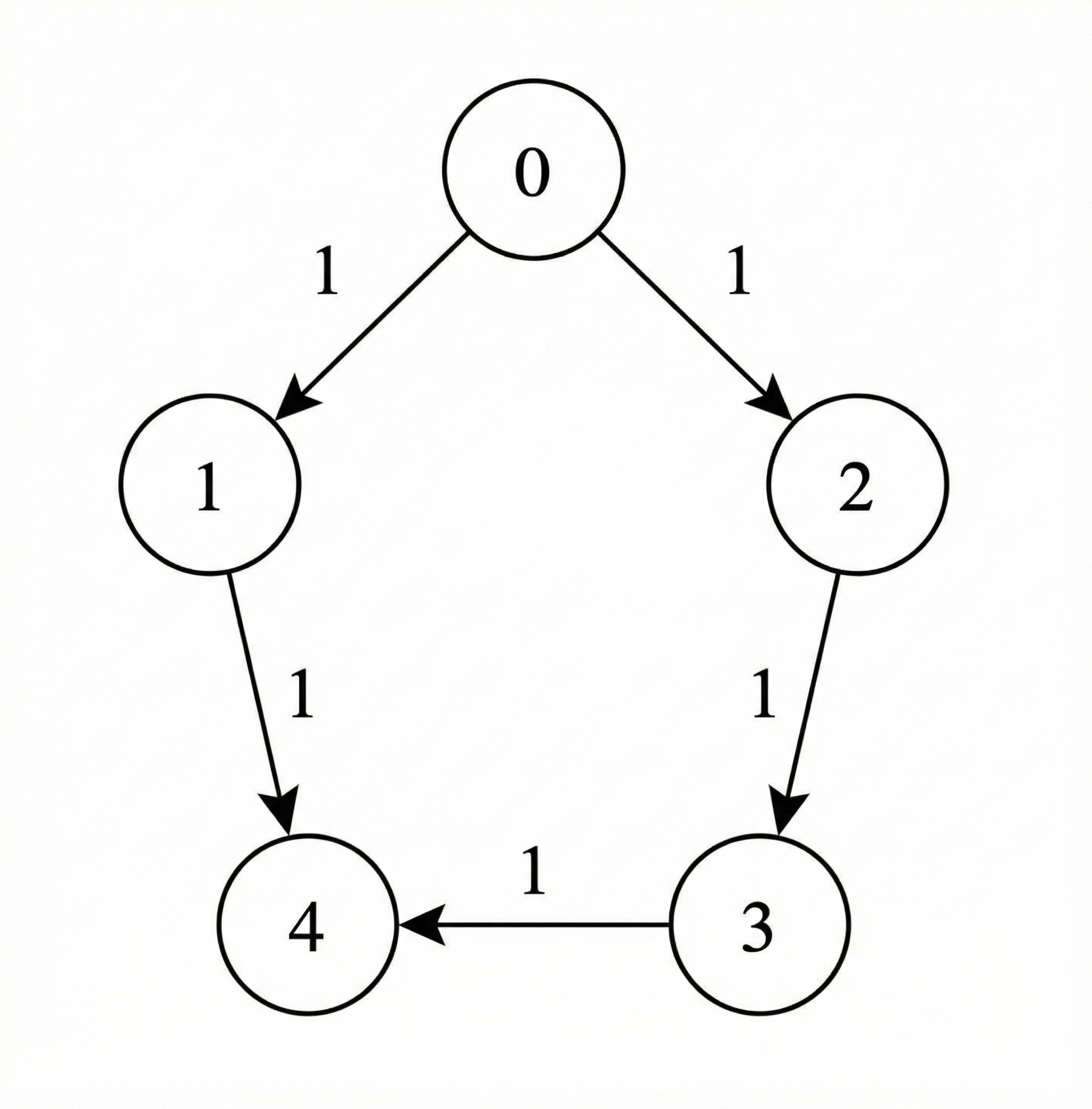
Input: n = 5, edges = [[0,1,1],[1,4,1],[0,2,1],[2,3,1],[3,4,1]], power = 4, cost = [2,3,1,1,1], source = 0, target = 4
Output: [3,0]
Explanation:
- The signal starts at node 0 with 4 units of power.
- The path
0 -> 1 -> 4is not valid, because after leaving node 0, the signal has 2 units of power remaining, which is less thancost[1] = 3. - The valid path
0 -> 2 -> 3 -> 4takes a total time of 3. - The total power consumed along this path is
cost[0] + cost[2] + cost[3] = 4, leaving 0 remaining power. - Hence, the answer is
[3, 0].
Example 2:
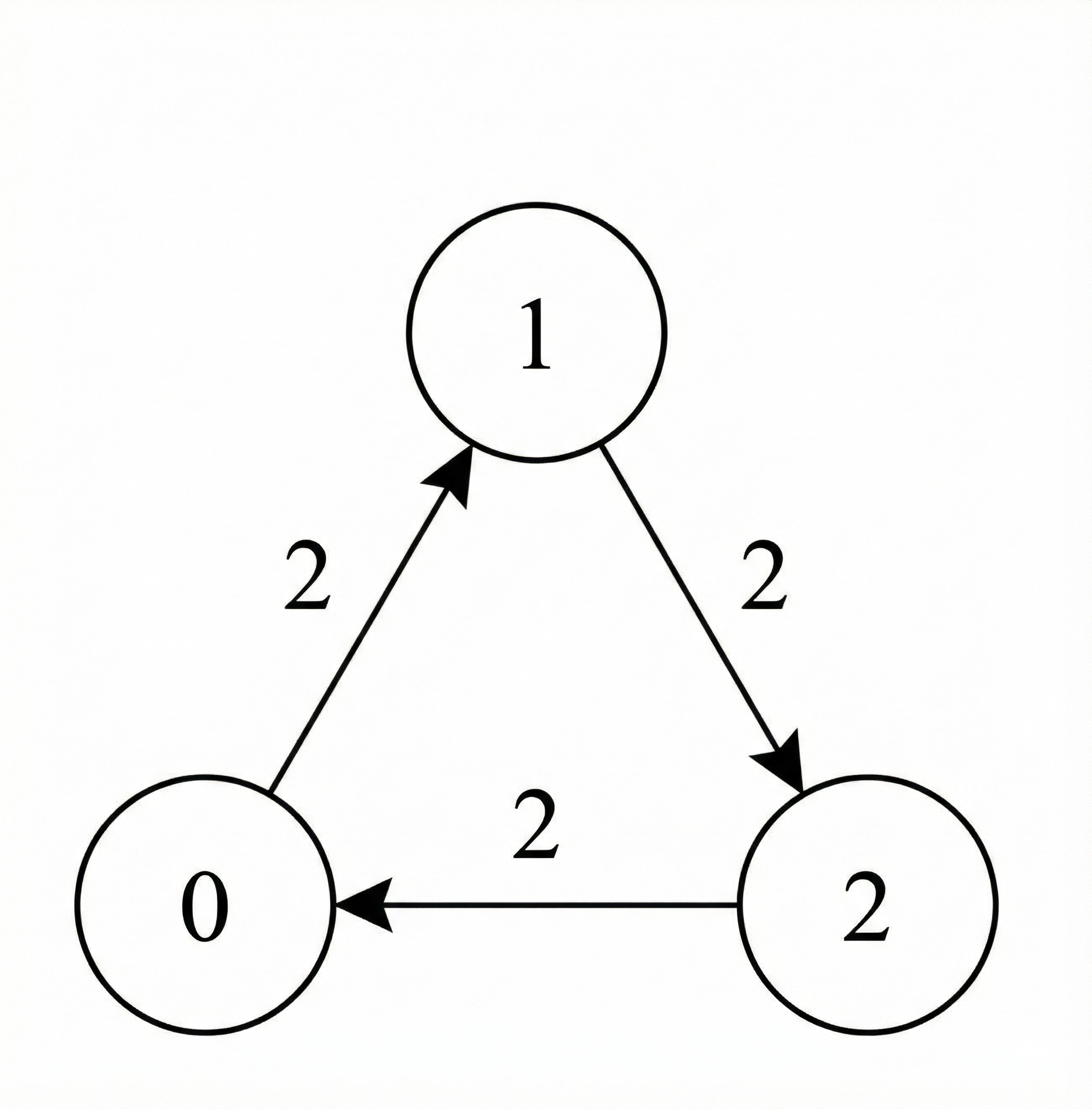
Input: n = 3, edges = [[0,1,2],[1,2,2],[2,0,2]], power = 3, cost = [1,1,1], source = 1, target = 1
Output: [0,3]
Explanation:
- Since the
sourceandtargetare the same node, no traversal is required. - Hence, the minimum total time taken is 0, and no power is consumed.
- Therefore, the answer is
[0, 3].
Example 3:
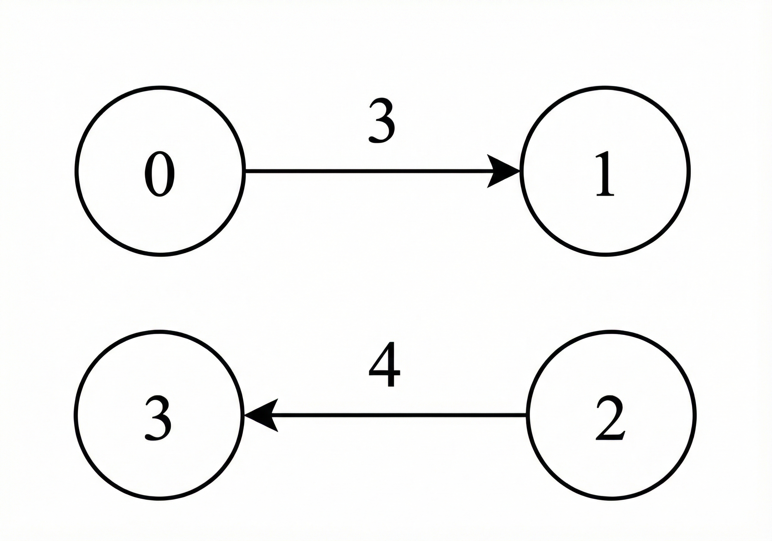
Input: n = 4, edges = [[0,1,3],[2,3,4]], power = 3, cost = [1,1,1,1], source = 0, target = 3
Output: [-1,-1]
Explanation:
There is no valid path from source to target, therefore return [-1, -1].
Constraints:
1 <= n <= 10000 <= edges.length <= 1000edges[i] = [ui, vi, ti]0 <= ui, vi <= n - 11 <= ti <= 1091 <= power <= 1000cost.length == n1 <= cost[i] <= 20000 <= source, target <= n - 1
Approach Overview
Problem Overview: You need to reach a target position while consuming a limited amount of power. Each move takes time and may reduce available power, so the goal is to find the path that reaches the target in the minimum time without exceeding the power limit.
Approach 1: Brute Force Path Exploration (Exponential Time)
Enumerate every possible sequence of moves from the starting state while tracking remaining power. Each state stores the current position, elapsed time, and remaining power. Use recursive exploration or a queue to generate all paths and discard those that exceed the power limit. This approach quickly becomes impractical because the number of possible paths grows exponentially with the graph or grid size. Time complexity is O(b^d) where b is branching factor and d is depth; space complexity is also O(b^d) due to stored states.
Approach 2: BFS with State Tracking (O(V * P + E * P))
If every move takes the same amount of time, treat the problem as a layered graph where each node is represented as (position, remainingPower). Perform a BFS starting from the initial state and push valid transitions that do not exceed the power limit. Maintain a visited structure to avoid revisiting the same state with equal or worse power. BFS guarantees the first time you reach the target is the minimum time under uniform edge weights. Time complexity is O((V + E) * P) and space complexity is O(V * P), where P is the maximum power.
Approach 3: Dijkstra's Algorithm with Extended State (Optimal for Weighted Moves)
When moves have different time costs, model the problem as a shortest-path search over a state graph. Each state becomes (node, remainingPower). Use a priority queue ordered by total time. From each state, iterate through possible transitions, update time, and subtract power cost. Push the new state into the heap only if it improves the best known time for that configuration. This technique combines ideas from graph algorithms and priority queues. Time complexity is O((V * P + E * P) log (V * P)) and space complexity is O(V * P). In practice this performs well because many dominated states are pruned.
Approach 4: Pruned Shortest Path with Dominance Optimization
You can reduce the search space by discarding states that are strictly worse than previously seen ones. If you reach the same node with less remaining power and higher time, that state can never lead to an optimal solution. Maintaining a best-time table per node and power level significantly cuts the number of pushes into the priority queue. The complexity remains O((V * P) log (V * P)) in the worst case but performs closer to linear exploration in practice.
Recommended for interviews: Start by explaining the brute force exploration to show you understand the constraints. Then move quickly to the shortest-path formulation where the state includes remaining power. Interviewers typically expect the Dijkstra with extended state approach because it handles weighted transitions and demonstrates familiarity with shortest path algorithms and state compression techniques.
Complexity Analysis
| Approach | Time | Space | When to Use |
|---|---|---|---|
| Brute Force Path Exploration | O(b^d) | O(b^d) | Only for understanding the search space or extremely small inputs |
| BFS with (node, power) State | O((V + E) * P) | O(V * P) | When each move has equal time cost |
| Dijkstra with Extended State | O((V * P + E * P) log (V * P)) | O(V * P) | General case with different time costs per move |
| Pruned Dijkstra (Dominance Check) | O((V * P) log (V * P)) | O(V * P) | Large inputs where many states can be dominated and pruned |