
Minimum Cost Tree From Leaf Values - Solution & Explanation
Problem Statement
Given an array arr of positive integers, consider all binary trees such that:
- Each node has either
0or2children; - The values of
arrcorrespond to the values of each leaf in an in-order traversal of the tree. - The value of each non-leaf node is equal to the product of the largest leaf value in its left and right subtree, respectively.
Among all possible binary trees considered, return the smallest possible sum of the values of each non-leaf node. It is guaranteed this sum fits into a 32-bit integer.
A node is a leaf if and only if it has zero children.
Example 1:
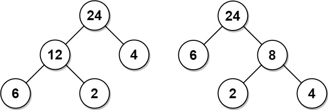
Input: arr = [6,2,4]
Output: 32
Explanation: There are two possible trees shown.
The first has a non-leaf node sum 36, and the second has non-leaf node sum 32.
Example 2:
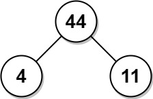
Input: arr = [4,11]
Output: 44
Constraints:
2 <= arr.length <= 401 <= arr[i] <= 15- It is guaranteed that the answer fits into a 32-bit signed integer (i.e., it is less than 231).
Approach Overview
Problem Overview: You are given an array where each value represents a leaf node in an in-order traversal of a binary tree. Every non-leaf node value equals the product of the maximum leaf values in its left and right subtrees. The task is to construct the tree with the minimum possible sum of all non-leaf node values.
Approach 1: Dynamic Programming (O(n³) time, O(n²) space)
This approach treats the problem similarly to matrix chain multiplication. Use a DP table dp[i][j] representing the minimum cost to build a tree from subarray arr[i..j]. For each range, try every possible partition k between i and j. The cost equals dp[i][k] + dp[k+1][j] + max(arr[i..k]) * max(arr[k+1..j]). Precompute maximum values for subarrays to avoid repeated scans. This solution demonstrates the optimal substructure clearly but becomes slow for larger inputs due to the cubic time complexity. Useful when learning interval dynamic programming patterns.
Approach 2: Greedy Monotonic Stack (O(n) time, O(n) space)
The optimal insight is that smaller leaves should be combined earlier to minimize multiplication cost. Use a decreasing monotonic stack. Iterate through the array and maintain elements in decreasing order. When the current value is greater than or equal to the stack top, pop the top element and add the cost mid * min(stackTop, current). This ensures each leaf pairs with the smallest possible larger neighbor, minimizing contribution to the total sum. After processing the array, multiply remaining adjacent stack elements until one element remains. The stack guarantees each element is pushed and popped once, giving linear complexity. This pattern frequently appears in problems involving nearest greater elements and stack-based greedy optimization.
Recommended for interviews: Start by explaining the dynamic programming formulation to show you understand the optimal substructure of the problem. Then move to the greedy monotonic stack solution, which reduces the complexity from O(n³) to O(n). Interviewers typically expect the stack-based approach because it demonstrates pattern recognition and optimization skills.
Approach 1: Dynamic Programming Approach
The Dynamic Programming approach aims to construct solutions to smaller instances of the problem and then use these solutions to build solutions for the larger problem. We will use a matrix `dp` where `dp[i][j]` represents the minimum cost to build a tree using the subarray `arr[i]` to `arr[j]`. For each possible subarray, we will calculate the cost of making each element in the range a root and update the `dp` matrix with the minimum values.
This Python solution uses a dynamic programming table `dp` with an auxiliary table `max_leaves` to store the maximum leaf node in any subarray. We iterate over subarray lengths, filling in the `dp` values based on smaller subproblems. We also calculate the minimal cost by considering every possible division `k` of the subarray and taking the minimum.
Complexity
Time Complexity: O(n^3) due to the nested loops over subarray lengths and possible splits.
Space Complexity: O(n^2) for the `dp` and `max_leaves` arrays.
Approach 2: Greedy Stack Approach
The Greedy Stack Approach involves using a stack to store leaf values in a manner that we can always efficiently compute the minimum possible non-leaf node sum at each step. By iteratively removing the smaller of the pair between any two adjacent elements and calculating it with its closest neighbor, we minimize the resulting non-leaf node sum, guaranteeing efficiency in computation.
This Python code uses a stack for leaf values, checking and resolving conditions by viewing the last element to improve the resulting non-leaf sum through the stack. We only calculate products amongst necessary consecutive nodes inevitably leading to efficient reductions.
Complexity
Time Complexity: O(n) due to single pass scanning and stack operations.
Space Complexity: O(n) for maintaining the stack of elements.
Approach 3: Memoization Search
According to the problem description, the values in the array arr correspond one-to-one with the values in the inorder traversal of each leaf node of the tree. We can divide the array into two non-empty sub-arrays, corresponding to the left and right subtrees of the tree, and recursively solve for the minimum possible sum of all non-leaf node values in each subtree.
We design a function dfs(i, j), which represents the minimum possible sum of all non-leaf node values in the index range [i, j] of the array arr. The answer is dfs(0, n - 1), where n is the length of the array arr.
The calculation process of the function dfs(i, j) is as follows:
- If
i = j, it means that there is only one element in the arrayarr[i..j], and there are no non-leaf nodes, sodfs(i, j) = 0. - Otherwise, we enumerate
k \in [i, j - 1], divide the arrayarrinto two sub-arraysarr[i..k]andarr[k + 1..j]. For eachk, we recursively calculatedfs(i, k)anddfs(k + 1, j). Here,dfs(i, k)represents the minimum possible sum of all non-leaf node values in the index range[i, k]of the arrayarr, anddfs(k + 1, j)represents the minimum possible sum of all non-leaf node values in the index range[k + 1, j]of the arrayarr. Sodfs(i, j) = min_{i leq k < j} {dfs(i, k) + dfs(k + 1, j) + max_{i leq t leq k} {arr[t]} max_{k < t leq j} {arr[t]}}.
In summary, we can get:
$
dfs(i, j) = \begin{cases}
0, & if  i = j \
min_{i leq k < j} {dfs(i, k) + dfs(k + 1, j) + max_{i leq t leq k} {arr[t]} max_{k < t leq j} {arr[t]}}, & if  i < j
\end{cases}
In the above recursive process, we can use the method of memoization search to avoid repeated calculations. Additionally, we can use an array g to record the maximum value of all leaf nodes in the index range [i, j] of the array arr. This allows us to optimize the calculation process of dfs(i, j):
dfs(i, j) = \begin{cases}
0, & if  i = j \
min_{i leq k < j} {dfs(i, k) + dfs(k + 1, j) + g[i][k] cdot g[k + 1][j]}, & if  i < j
\end{cases}
Finally, we return dfs(0, n - 1).
The time complexity is O(n^3), and the space complexity is O(n^2). Here, n is the length of the array arr$.
Code
Python
Java
C++
Go
TypeScript
Approach 4: Dynamic Programming
We can change the memoization search in Solution 1 to dynamic programming.
Define f[i][j] to represent the minimum possible sum of all non-leaf node values in the index range [i, j] of the array arr, and g[i][j] to represent the maximum value of all leaf nodes in the index range [i, j] of the array arr. Then, the state transition equation is:
$
f[i][j] = \begin{cases}
0, & if  i = j \
min_{i leq k < j} {f[i][k] + f[k + 1][j] + g[i][k] cdot g[k + 1][j]}, & if  i < j
\end{cases}
Finally, we return f[0][n - 1].
The time complexity is O(n^3), and the space complexity is O(n^2). Here, n is the length of the array arr$.
Code
Python
Java
C++
Go
TypeScript
Approach 5: Default Approach
Code
Python
Complexity Comparison
| Approach | Complexity |
|---|---|
| Dynamic Programming Approach | Time Complexity: O(n^3) due to the nested loops over subarray lengths and possible splits. |
| Greedy Stack Approach | Time Complexity: O(n) due to single pass scanning and stack operations. |
| Memoization Search | — |
| Dynamic Programming | — |
| Default Approach | — |
Detailed Complexity Analysis
| Approach | Time | Space | When to Use |
|---|---|---|---|
| Dynamic Programming (Interval DP) | O(n³) | O(n²) | When demonstrating interval DP reasoning or solving small input sizes |
| Greedy Monotonic Stack | O(n) | O(n) | Best choice for interviews and production due to linear performance |
Video Solution
Lecture 129: Minimum Cost Tree From Leaf Values || DP Series • CodeHelp - by Babbar • 37,810 views views
Watch 9 more video solutions →Frequently Asked Questions
Is Minimum Cost Tree From Leaf Values easy or hard?
Minimum Cost Tree From Leaf Values Python/Java solution
How to solve Minimum Cost Tree From Leaf Values in O(n)?
What is the best approach for Minimum Cost Tree From Leaf Values?
Is Minimum Cost Tree From Leaf Values asked at Google/Amazon/Meta?
What data structure is used in Minimum Cost Tree From Leaf Values?
What is the time complexity of Minimum Cost Tree From Leaf Values?
Ready to solve this problem?
Practice Minimum Cost Tree From Leaf Values with our built-in code editor and test cases.
Practice on FleetCode